4. Logic — Development v0.0

4.1. Logic symbols¶

Some logical symbols used in this documentation. See also List of logic symbols on Wikipedia.

Symbol	Text	Name	Alternatives
$\neg$	`!`	NOT	$\sim$
$\wedge$	`&`	AND
$\vee$	`\|`	OR
$\to$	`->`	IF
$\leftrightarrow$	`<->`	IFF	$\Leftrightarrow$, $\equiv$
$\veebar$	`^`	XOR	$\oplus$, $\not\leftrightarrow$, $\not\equiv$
$\uparrow$	`!&`	NAND
$\downarrow$	`!\|`	NOR
$\bot$	`F`	FALSE	`0`
$\top$	`T`	TRUE	`1`

4.2. Notation¶

For index notation of sequences, e.g.:

\[\mathop{(x_k)}_{k=0}^{n-1} = {(x_k)}_{k=0}^{n-1} = (x_0, x_1, \dotsc, x_{n-1})\]

see article Indexing. For mathematical families in general see Indexed family or Familie (German).

For functions, see Notation for functions and Table of symbols for functions (German).

4.3. Combinatorics¶

Fundamental logic is mainly governed by variations without repetition (or n-sequences in X [1]):

When the ordering of objects matters, and an object can be chosen more than once, we are talking about variations with repetition, and the number of variations is:

\[c^n\]

where $c$ is the number of objects from which you can choose and $n$ is the number of objects we can choose (repetitions allowed). (Source: Variations with repetition)

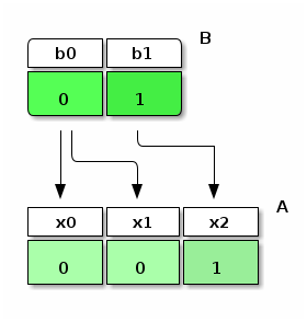
Distributing $c=2$ balls from a sequence $B=(b_0,b_1)=(0,1),$ to $n$ boxes $x_k$, results in a distribution

\[A=\mathop{(x_k)}_{k=0}^{n-1} .\]

Since order matters and there can be more boxes than unique balls are available, the distribution must be variations with repetition. The following figure shows an example for distributing $c=2$ balls to $n=3$ boxes:

$@startditaa /------+------\ B | b0 | b1 | +------+------+ | c5F5 | c4E4 | | 0 | 1 | \------+------/ || | || \------+ |\-----\ | | | | v v v +------+------+------+ A | x0 | x1 | x2 | +------+------+------+ | cAFA | cAFA | c9E9 | | 0 | 0 | 1 | +------+------+------+ @endditaa$

For $c=|B|=2$ balls and $n=|A|$ boxes, the total number of possible variations $A_j$ is $c^n$. The sequence $X$ of variations $A_j$ is then

\[X = \mathop{(A_j)}_{j=0}^{2^n-1} .\]

The following figure shows an example for $n=3 \Rightarrow |X|=8$:

Correlating each distribution $A_j$ to a new box $y_j$ generates a sequence of boxes

\[Y = \mathop{(y_j)}_{j=0}^{2^n-1},\]

The number of possible distributions for $2$ balls to boxes $y_j$ is $2^{|Y|} = 2^{2^n}$, which generates a sequence of distributions

\[F = \mathop{(Y_i)}_{i=0}^{2^{2^n}-1} .\]

The following figure shows an example for $n=3 \Rightarrow |A|=8 \Rightarrow |F|=256$:

4.4. Boolean functions and truth tables¶

Quoting from article Boolean function:

In mathematics and logic, a (finitary) Boolean function (or switching function) is a function of the form $ƒ : B^{\,n} \rightarrow B$, where $B = (0, 1)$ is a Boolean domain and $n$ is a non-negative integer called the arity of the function. In the case where $n = 0$, the “function” is essentially a constant element of $B$.

Every $n$-ary Boolean function can be expressed as a propositional formula in $n$ variables $x_0, \dotsc, x_n$.

Boolean functions are classified by arity $n \in \mathbb{N}_0$ as $f^n : B^{\,n} \to B^{\,1}$, such that each function $f^n$ maps a sequence $A=\mathop{(x_k)}_{k=0}^{n-1}$ of $n$ values $x_k \in B$ to a single value $y \in B$:

\[f^n : A \mapsto y .\]

The number of possible variations for $A$ is $|(B \rightarrow A)| = |B|^{|A|} = 2^n$, which generates the sequence of possible input variations

\[X=\mathop{\left(A_j\right)}_{j=0}^{2^n-1} ,\]

and the corresponding sequence of output values

\[Y=\mathop{(y_j)}_{j=0}^{2^n-1} .\]

The number of possible output sequences is $|(B \rightarrow Y)| = |B|^{|Y|} = 2^{2^n}$. Therefore the sequence $F^n$ of $n$-ary Boolean functions is

\[\begin{split}F^n = {\left(f^{n}_{i} \left| \begin{split} f^{n}_{i} :\,& X \rightarrow Y_i,\\ &A_j \mapsto y_j\\ \end{split} \right. \right)}_{i=0}^{2^{2^n}-1} .\end{split}\]

A truth table defines a function $f^n_i$ by specifying an output value $y_j$ for each combination $A_j$ of input values $x_k$.

4.4.1. Universal lookup function¶

The order of sequences $F^n, X, Y$ is defined such that each truth table row $j$

\[f^n_i(A_j) = y_j\]

can be calculated independently given arity $n$, function index $i$ and output value index $j$.

Function $\mathrm{bin}(d,m)$ converts an integer $d$ into a sequence of binary digits:

\[\mathrm{bin}(d,m) : d \mapsto (b_e|b_e = \left\lfloor\frac{d}{2^{m-1-e}}\right\rfloor \bmod 2)_{e=0}^{m-1}, d \in \mathbb{N}_0, b_e \in B .\]

The sequence of output values $Y_i$ for $f^n_i$ is generated by

\[Y_i = \mathrm{bin}(i, 2^n) .\]

The truth table row $j$ is then defined by

\[f^n_i(A_j) = Y_{i_j} .\]

Given $f^{3}_{23}$, the sequence of ouptut values $Y_{23}$ is $(0,0,0,1,0,1,1,1)$ and truth table row $j=3$ is then defined by $f^{3}_{23}(0, 1, 1) = 1$. The follwing table shows the complete complete truth table for $f^{3}_{23}$:

$k \rightarrow$	0	1	2
$j \downarrow$	$x_0$	$x_1$	$x_2$	$f^{3}_{23}$
0	0	0	0	0
1	0	0	1	0
2	0	1	0	0
3	0	1	1	1
4	1	0	0	0
5	1	0	1	1
6	1	1	0	1
7	1	1	1	1

4.4.2. Nullary Boolean functions¶

These are the truth constants from $B$ expressed as functions $(f^0_i())_{i=0}^1$ without parameters.

$f^{0}_{0}$	$f^{0}_{1}$
$\bot$	$\top$
0	1

4.4.3. Unary Boolean functions¶

	$f^{1}_{0}$	$f^{1}_{1}$	$f^{1}_{2}$	$f^{1}_{3}$
$p$	$\bot$	$p$	$\neg p$	$\top$
0	0	0	1	1
1	0	1	0	1

4.4.4. Binary Boolean functions¶

		$f^{2}_{0}$	$f^{2}_{1}$	$f^{2}_{2}$	$f^{2}_{3}$	$f^{2}_{4}$	$f^{2}_{5}$	$f^{2}_{6}$	$f^{2}_{7}$	$f^{2}_{8}$	$f^{2}_{9}$	$f^{2}_{10}$	$f^{2}_{11}$	$f^{2}_{12}$	$f^{2}_{13}$	$f^{2}_{14}$	$f^{2}_{15}$
$p$	$q$	$\bot$	$\wedge$	$\not\to$	$p$	$\not\leftarrow$	$q$	$\veebar$	$\vee$	$\downarrow$	$\leftrightarrow$	$\neg q$	$\leftarrow$	$\neg p$	$\rightarrow$	$\uparrow$	$\top$
0	0	0	0	0	0	0	0	0	0	1	1	1	1	1	1	1	1
0	1	0	0	0	0	1	1	1	1	0	0	0	0	1	1	1	1
1	0	0	0	1	1	0	0	1	1	0	0	1	1	0	0	1	1
1	1	0	1	0	1	0	1	0	1	0	1	0	1	0	1	0	1

4.5. Mask operation¶

Let $m, d, b \in B$, let $g^1_c \in F^1$ be an arbitrary unary logical function. Then an operation $\mbox{O}_{\mbox{mask}} : B^{\,2} \to B^{\,1}$ is a mask operation, iff for all combinations of input bits $\mathop{\left((m, d)_j\right)}_{j=0}^{2^2}$ there exists a constant $b$ so that function $f^2_i(m, d) = d$, if $m = b$, and $f^2_i(m, d) = g^1_c(d)$, if $m = \neg b$.

\[\begin{split}\mbox{O}_{\mbox{mask}}: B^{\,2} \to B^{\,1} \Leftrightarrow \forall m, d\, \exists b : f^2_i(m, d) = \left\{ \begin{array}{ll} d & \mbox{if}\,\, m = b\\ g^1_c(d) & \mbox{if}\,\, m = \neg b \end{array} \right.\end{split}\]

Truth table, using $p$ as mask bit, $q$ as data bit:

		$f^{2}_{0}$	$f^{2}_{1}$	$f^{2}_{2}$	$f^{2}_{3}$	$f^{2}_{4}$	$f^{2}_{5}$	$f^{2}_{6}$	$f^{2}_{7}$	$f^{2}_{8}$	$f^{2}_{9}$	$f^{2}_{10}$	$f^{2}_{11}$	$f^{2}_{12}$	$f^{2}_{13}$	$f^{2}_{14}$	$f^{2}_{15}$
$m$	$d$	$\bot$	$\wedge$	$\not\to$	$m$	$\not\leftarrow$	$d$	$\veebar$	$\vee$	$\downarrow$	$\leftrightarrow$	$\neg d$	$\leftarrow$	$\neg m$	$\rightarrow$	$\uparrow$	$\top$
0	0	0	0	0	0	0	0	0	0	1	1	1	1	1	1	1	1
0	1	0	0	0	0	1	1	1	1	0	0	0	0	1	1	1	1
1	0	0	0	1	1	0	0	1	1	0	0	1	1	0	0	1	1
1	1	0	1	0	1	0	1	0	1	0	1	0	1	0	1	0	1

Only those functions qualify as candidates for mask operations, which either have 2 entries for $f^2_i(m, d)$ with $f^2_i(0, 0) = 0$ and $f^2_i(0, 1) = 1$, or 2 entries with $f^2_i(1, 0) = 0$ and $f^2_i(1, 1) = 1$:

		$f^{2}_{1}$	$f^{2}_{4}$	$f^{2}_{5}$	$f^{2}_{6}$	$f^{2}_{7}$	$f^{2}_{9}$	$f^{2}_{13}$
$m$	$d$	$\wedge$	$\not\leftarrow$	$d$	$\veebar$	$\vee$	$\leftrightarrow$	$\rightarrow$
0	0	0	0	0	0	0	1	1
0	1	0	1	1	1	1	0	1
1	0	0	0	0	1	1	0	0
1	1	1	0	1	0	1	1	1

4.5.1. Clearing data bits¶

$f^{2}_{1}$ (AND) allows clearing data bits by setting the corresponding mask value to 0. For mask values of 1, the data bits remain unmodified ($b=1, g^1_c=f^{1}_{0}$):

MASK	1	1	0	0	1	1	0	0
DATA	0	1	1	1	0	1	0	1
AND	$\downarrow$	$\downarrow$	$\downarrow$	$\downarrow$	$\downarrow$	$\downarrow$	$\downarrow$	$\downarrow$
RES	0	1	0	0	0	1	0	0

4.5.2. Setting data bits¶

$f^{2}_{7}$ (OR) allows setting data bits by setting the corresponding mask value to 1. For mask values of 0, the data bits remain unmodified ($b=0, g^1_c=f^{1}_{3}$):

MASK	0	0	1	1	0	0	1	1
DATA	0	1	1	1	0	1	0	1
OR	$\downarrow$	$\downarrow$	$\downarrow$	$\downarrow$	$\downarrow$	$\downarrow$	$\downarrow$	$\downarrow$
RES	0	1	1	1	0	1	1	1

4.5.3. Inverting data bits¶

$f^{2}_{6}$ (XOR) allows inverting data bits by setting the corresponding mask value to 1. For mask values of 0, the data bits remain unmodified ($b=0, g^1_c=f^{1}_{2}$):

MASK	0	0	1	1	0	0	1	1
DATA	0	1	1	1	0	1	0	1
XOR	$\downarrow$	$\downarrow$	$\downarrow$	$\downarrow$	$\downarrow$	$\downarrow$	$\downarrow$	$\downarrow$
RES	0	1	0	0	0	1	1	0

Special mask operations are:

\[\begin{split}\begin{array}{llll} \hphantom{\neg}f^{2}_{6}(m, \hphantom{\neg}m) & = & \hphantom{\neg}(m \veebar \hphantom{\neg}m) & = 0\\ \hphantom{\neg}f^{2}_{6}(m, \neg m) & = & \hphantom{\neg}(m \veebar \neg m) & = 1\\ \neg f^{2}_{6}(m, \hphantom{\neg}m) & = & \neg (m \veebar \hphantom{\neg}m) & = 1 \end{array}\end{split}\]

4.5.4. Other mask operations¶

The other mask operations can all be expressed in terms of AND, OR, XOR.

$f^{2}_{4}$ allows clearing data bits by setting the corresponding mask value to 1. For mask values of 0, the data bits remain unmodified ($b=0, g^1_c=f^{1}_{0}$). This can simply be replaced by inverting the mask bits and performing an AND operation:

\[f^{2}_{4}(m, d) = f^{2}_{1}(\neg m, d) = \neg m \wedge d\]

$f^{2}_{5}$ leaves all data bits unmodified ($b=0, g^1_c=f^{1}_{1}$ and $b=1, g^1_c=f^{1}_{1}$). It is therefore really a NOOP, i.e., just using the data bits is sufficient. However, to fulfill the requirements of a binary operation with arbitrary mask bits, any mask operation can be used by transforming the mask so as to leave the data bits unmodified.

\[\begin{split}\begin{array}{lllll} f^{2}_{5}(m, d) & = f^{2}_{1}(f^{2}_{6}(m,\neg m), d) & = (m \veebar \neg m) \wedge d & = 1 \wedge d\\ f^{2}_{5}(m, d) & = f^{2}_{7}(f^{2}_{6}(m,\hphantom{\neg}m), d) & = (m \veebar \hphantom{\neg}m) \vee d & = 0 \vee d\\ f^{2}_{5}(m, d) & = f^{2}_{6}(f^{2}_{6}(m,\hphantom{\neg}m), d) & = (m \veebar \hphantom{\neg}m) \veebar d & = 0 \veebar d \end{array}\end{split}\]

$f^{2}_{9}$ (IFF) allows inverting data bits by setting the corresponding mask value to 0. For mask values of 1, the data bits remain unmodified ($b=1, g^1_c=f^{1}_{2}$). This can be achieved, by inverting the mask for $f^{2}_{7}$:

\[f^{2}_{9}(m, d) = f^{2}_{7}(\neg m, d) = \neg m \veebar d\]

$f^{2}_{13}$ allows setting data bits by setting the corresponding mask value to 0. For mask values of 1, the data bits remain unmodified ($b=1, g=f^{1}_{3}$). This can be achieved by inverting the mask for $f^{2}_{6}$:

\[f^{2}_{13}(m, d) = f^{2}_{6}(\neg m, d) = \neg m \vee d\]

4.6. Functional completeness¶

See Truth Function, section Functional completeness and main article Functional completeness.
See also “You cannot NOT have NOT” in Is XOR a combination of AND and NOT operators?.

It is established that functions NOT and AND are sufficient to generate all other binary logical functions. Since function AND can be generated with functions NOT and OR:

\[\begin{split}\begin{array}{ll} &(p \wedge q)\\ =&\neg(\neg(p \wedge q)))\\ =&\neg(\neg p \vee \neg q), \end{array}\end{split}\]

functions NOT and OR are also functionally complete.

When looking for a single binary Boolean function that is functionally complete, candidates are all functions that generate a unary NOT: $f^2_i(p,p) = \neg p$:

		$f^{2}_{8}$	$f^{2}_{10}$	$f^{2}_{12}$	$f^{2}_{14}$
$p$	$q$	$\downarrow$	$\neg q$	$\neg p$	$\uparrow$
0	0	1	1	1	1
1	1	0	0	0	0

this identifies $f^{2}_{8}$ (NOR), $f^{2}_{10}$ ($\neg q$), $f^{2}_{12}$ ($\neg p$), $f^{2}_{14}$ (NAND).

Functions $f^{2}_{10}$ and $f^{2}_{12}$ are actually unary functions, each ignoring one of the inputs while negating the other. Since they are equivalent to a unary negation, they cannot be functionally complete, as NOT by itself is not functionally complete.

		$f^{2}_{10}$	$f^{2}_{12}$
$p$	$q$	$\neg q$	$\neg p$
0	0	1	1
0	1	0	1
1	0	1	0
1	1	0	0

However, functions $f^{2}_{8}$ (NOR) and $f^{2}_{14}$ (NAND) are already very close to the functions AND and OR. Both provide NOT via $f^2_{8}(p,p) = f^2_{14}(p,p) = \neg p$ as shown above.

		$f^{2}_{8}$	$f^{2}_{14}$
$p$	$q$	$\downarrow$	$\uparrow$
0	0	1	1
0	1	0	1
1	0	0	1
1	1	0	0

$f^{2}_{8}$ (NOR) can be used to express $f^{2}_{7}$ (OR) as:

\[\begin{split}\begin{array}{ll} \neg p &= p \downarrow p\\ p \vee q &= \neg ( p \downarrow q )\\ p \vee q &= ( p \downarrow q ) \downarrow ( p \downarrow q ), \end{array}\end{split}\]

which makes $f^{2}_{8}$ functionally complete.

$f^{2}_{14}$ (NAND) can be used to express $f^{2}_{1}$ (AND) as:

\[\begin{split}\begin{array}{ll} \neg p &= p \uparrow p\\ p \wedge q &= \neg ( p \uparrow q )\\ p \wedge q &= ( p \uparrow q ) \uparrow ( p \uparrow q ), \end{array}\end{split}\]

which makes $f^{2}_{14}$ functionally complete.

For $\{\mathrm{AND}, \mathrm{XOR}, \top\}$, negation can be expressed as:

\[\neg p = \top \veebar p.\]

The resulting set of functions $\{\mathrm{AND}, \mathrm{XOR}, \top, \mathrm{NOT}\}$ is a superset of the functionally complete set $\{\mathrm{AND}, \mathrm{NOT}\}$, and therefore also functionally complete.

4.6.1. Composition of Boolean functions with NOT and AND¶

Proposition: All Boolean functions in $F^n, n \in \mathbb{N}_0$ can be composed from Boolean functions $f^{1}_{2}$ aka ( NOT , $\neg$ ) and $f^{2}_{1}$ aka ( AND , $\wedge$ ).

4.6.1.1. Composing nullary functions from NOT and AND¶

Article Truth Function argues that only functions in $F^m, m \in \mathbb{N}$ can be composed.

However, the nullary function $f^{0}_{0}$ aka ( FALSE , F , $\bot$ ) is quite obviously equivalent to all functions $f^m_0$ for all combinations of input values $((x_k)_j)$:

\[f^{m}_{0}(x_0, x_1, \dotsc, x_{m-1}) = f^{m-1}_{0}(x_0, x_1, \dotsc, x_{m-2}) .\]

So any function $f^{m}_{0}$ with arbitrary input values can always be reduced to $f^{0}_{0}$:

\[f^{2}_{0}(p, q) = f^{1}_{0}(p) = f^{0}_{0}().\]

When trying to expand a function $f^{n}_{0}$ to $f^{n+1}_{0}$, the problem arises, where the input variables should come from:

\[f^{0}_{0}() = f^{1}_{0}(\dotsc) = f^{2}_{0}(\dotsc) .\]

An obvious choice would be constant values, which avoids inventing arbitrary variables:

\[f^{0}_{0}() = f^{1}_{0}(0) = f^{2}_{0}(0,0) .\]

Another possibility is using a variable symbol like $\phi$, that is not generally used:

\[f^{0}_{0}() = f^{1}_{0}(\phi) = f^{2}_{0}(\phi, \phi) ,\]

which makes all functions $f^n_0$ equivalent:

\[f^{n}_{0}(x_0, x_1, \dotsc, x_{n-1}) = f^{n+1}_{0}(x_0, x_1, \dotsc, x_{n-1}, \phi) .\]

Therefore $f^0_0$ is proved expressable by a set of functions if any representative $f^{n}_{0}$ can be composed.

$f^{1}_{0}$ and $f^{2}_{0}$ can be defined by NOT and AND in various ways, which are all equivalent t0 $f^{0}_{0}$:

\[\begin{split}\begin{array}{lll} f^{1}_{0}(p) &= f^{2}_{1}(p,f^{1}_{2}(p)) &= p \wedge \neg p,\\ f^{2}_{0}(p, q) &= f^{2}_{1}(f^{2}_{1}(p,q),f^{1}_{2}(f^{2}_{1}(p,q))) &= (p \wedge q ) \wedge \neg (p \wedge q ),\\ &= f^{1}_{0}(f^{2}_{1}(p,q)) &= (p \wedge q ) \wedge \neg (p \wedge q ),\\ &= f^{2}_{1}(f^{1}_{0}(p),f^{1}_{0}(q)) &= (p \wedge \neg p) \wedge (q \wedge \neg q),\\ &= f^{2}_{1}(p,f^{1}_{0}(q)) &= p \wedge (q \wedge \neg q),\\ &= f^{2}_{1}(f^{1}_{0}(p),q) &= (p \wedge \neg p) \wedge q . \end{array}\end{split}\]

The expression

\[f^{2}_{1}(\phi,f^{1}_{2}(\phi))\]

is used to expand $f^0_0$. This ensures that the full expansion of a formula contains only the functions $f^1_2$ and $f^2_1$, formally satisfying functional completeness.

Trivially the nullary function $f^{0}_{1}$ aka ( TRUE , T , $\top$ ) is defined as negation of $f^{0}_{0}$:

\[f^{0}_{1} = f^{1}_{2}(f^{0}_{0}()) = \neg \bot = \top .\]

4.6.1.2. Convenience definition of OR¶

It is convenient to use $f^{2}_{7}$ aka ( OR , $\vee$ ) in addition to NOT and AND, so this is proved first by induction over the complete truth table:

\[\begin{split}&p \vee q = \neg ( \neg ( p \vee q )) = \neg ( \neg p \wedge \neg q )\\ &f^{2}_{7}(p,q) = f^{1}_{2}( f^{2}_{1}( f^{1}_{2}(p), f^{1}_{2}(q) ) )\end{split}\]

$p$	$q$	$\neg p$	$\neg q$	$\neg p \wedge \neg q$	$\neg(\neg p \wedge \neg q)$	$f^{2}_{7}(p,q), \vee$
0	0	1	1	1	0	0
0	1	1	0	0	1	1
1	0	0	1	0	1	1
1	1	0	0	0	1	1

4.6.2. Universal composition function¶

It is obvious, that a truth table for a Boolean function $f^m_i(x_0, x_1, \dotsc, x_{m-1})$ can be partitioned into an upper half, where $x_0=0$ and a lower half, where $x_0=1$. Each half without $x_0$ is then a truth table for a function $f^{m-1}_u(x_1, \dotsc, x_{m-1})$ and a function $f^{m-1}_v(x_1, \dotsc, x_{m-1})$ of arity $m-1$, $u,v \in (0, 1, \dotsc, 2^{2^{m-1}}-1), z \in (0, 1, \dotsc, 2^{2^{m}}-1)$. E.g.:

The composition function for $m > 1$

\[\begin{split}c^m_i : B^{\,m} \to B^{\,1}, c^m_i(x_0, x_1, \dotsc, x_k) = \left\{ \begin{array}{ll} f^{m-1}_{u}(x_1, \dotsc, x_k) & \mbox{if}\,\, x_0 = 0\\ f^{m-1}_{v}(x_1, \dotsc, x_k) & \mbox{if}\,\, x_0 = 1 ,\\ \end{array} \right.\end{split}\]

and the composition function for $m = 1$

\[\begin{split}c^1_z : B \to B, c^1_z(x_0) = \left\{ \begin{array}{ll} f^{0}_{u}() = Y_{z_0} & \mbox{if}\,\, x_0 = 0\\ f^{0}_{v}() = Y_{z_1} & \mbox{if}\,\, x_0 = 1 ,\\ \end{array} \right.\end{split}\]

can be expressed in terms of logical operators $\{ \bot, \top, \mathrm{NOT}, \mathrm{AND}, \mathrm{OR} \}$:

\[\begin{split}c^m_i(x_0, x_1, \dotsc, x_k) &~= ( \neg x_0 \wedge f^{m-1}_{u}(x_1, \dotsc, x_k) ) \vee ( x_0 \wedge f^{m-1}_{v}(x_1, \dotsc, x_k) ) ,\\ c^1_z(x_0) &~= ( \neg x_0 \wedge f^{0}_{u}() ) \vee ( x_0 \wedge f^{0}_{v}() ) .\\\end{split}\]

This is equivalent to the functional notation

\[\begin{split}c^m_i(x_0, x_1, \dotsc, x_k) &~= f^{2}_{7}( f^{2}_{1}( f^{1}_{2}(x_0), f^{m-1}_{u}(x_1, \dotsc, x_k) ), f^{2}_{1}( x_0, f^{m-1}_{v}(x_1, \dotsc, x_k) ) ),\\ c^1_z(x_0) &~= f^{2}_{7}( f^{2}_{1}( f^{1}_{2}(x_0), f^{0}_{u}() ), f^{2}_{1}( x_0, f^{0}_{v}() ) .\end{split}\]

Therefore the composition mechanism $c^m_i$ can be applied recursively to define any required Boolean function. The recursion is guaranteed to terminate at a function $c^1_z$, which only uses the previously defined functions $f^{0}_{0}$ aka ( FALSE , F , $\bot$ ), $f^{0}_{1}$ aka ( TRUE , T , $\top$ ), $f^{1}_{2}$ aka ( NOT , $\neg$ ), $f^{2}_{1}$ aka ( AND , $\wedge$ ), $f^{2}_{7}$ aka ( OR , $\vee$ ).

4.6.2.1. Unary functions defined by composition function¶

The unary funtions $f^{1}_{i}$ for example, are such defined as:

\[\begin{split}f^1_0(p) &= f^{2}_{7}( f^{2}_{1}( f^{1}_{2}(p), f^{0}_{0}() ), f^{2}_{1}( p, f^{0}_{0}() ) ), \\ f^1_1(p) &= f^{2}_{7}( f^{2}_{1}( f^{1}_{2}(p), f^{0}_{0}() ), f^{2}_{1}( p, f^{0}_{1}() ) ), \\ f^1_3(p) &= f^{2}_{7}( f^{2}_{1}( f^{1}_{2}(p), f^{0}_{1}() ), f^{2}_{1}( p, f^{0}_{1}() ) ) .\end{split}\]

Substituting $\bot$ for $f^{0}_{0}()$ and $\top$ for $f^{0}_{1}()$ gives:

\[\begin{split}f^1_0(p) &= f^{2}_{7}( f^{2}_{1}( f^{1}_{2}(p), \bot ), f^{2}_{1}( p, \bot ) ), \\ f^1_1(p) &= f^{2}_{7}( f^{2}_{1}( f^{1}_{2}(p), \bot ), f^{2}_{1}( p, \top ) ), \\ f^1_3(p) &= f^{2}_{7}( f^{2}_{1}( f^{1}_{2}(p), \top ), f^{2}_{1}( p, \top ) ) .\end{split}\]

Applying $p \wedge \bot = \bot$ and $p \wedge \top = p$ gives:

\[\begin{split}f^1_0(p) &= f^{2}_{7}( \bot, \bot ), \\ f^1_1(p) &= f^{2}_{7}( \bot, p ), \\ f^1_3(p) &= f^{2}_{7}( f^{1}_{2}(p), p ) .\end{split}\]

Finally applying $p \vee \bot = p$ and $p \vee \neg p = \top$ gives:

\[\begin{split}f^1_0(p) &= \bot \\ f^1_1(p) &= p \\ f^1_3(p) &= \top .\end{split}\]

4.6.2.2. Example composition function for $f^3_{23}$¶

\[\begin{split}c^3_{23}(x_0, x_1, x_2) = f^{2}_{7}( &f^{2}_{1}( f^{1}_{2}(x_0), f^{2}_{7}(f^{2}_{1}( f^{1}_{2}(x_1), f^{2}_{7}(f^{2}_{1}( f^{1}_{2}(x_2), f^{0}_{0}() ), f^{2}_{1}( x_2, f^{0}_{0}() )) ), f^{2}_{1}( x_1, f^{2}_{7}(f^{2}_{1}( f^{1}_{2}(x_2), f^{0}_{0}() ), f^{2}_{1}( x_2, f^{0}_{1}() )) )) ),\\ &f^{2}_{1}( x_0, f^{2}_{7}(f^{2}_{1}( f^{1}_{2}(x_1), f^{2}_{7}(f^{2}_{1}( f^{1}_{2}(x_2), f^{0}_{0}() ), f^{2}_{1}( x_2, f^{0}_{1}() )) ), f^{2}_{1}( x_1, f^{2}_{7}(f^{2}_{1}( f^{1}_{2}(x_2), f^{0}_{1}() ), f^{2}_{1}( x_2, f^{0}_{1}() )) )) )) .\end{split}\]

Optimized:

\[\begin{split}\begin{array}{llll} c^3_{23}(x_0, x_1, x_2) &~= f^{2}_{7}( &f^{2}_{1}( f^{1}_{2}(x_0), f^{2}_{7}(f^{2}_{1}( f^{1}_{2}(x_1), f^{0}_{0}() ), f^{2}_{1}( x_1, x_2 )) ), & |~\mbox{subst}~\bot, \top\\ &&f^{2}_{1}( x_0, f^{2}_{7}(f^{2}_{1}( f^{1}_{2}(x_1), x_2 ), f^{2}_{1}( x_1, f^{0}_{1}() )) ))\\ &~= f^{2}_{7}( &f^{2}_{1}( f^{1}_{2}(x_0), f^{2}_{7}(f^{2}_{1}( f^{1}_{2}(x_1), \bot ), f^{2}_{1}( x_1, x_2 )) ), & \left|~p \wedge \bot = \bot, p \wedge \top = p\right.\\ &&f^{2}_{1}( x_0, f^{2}_{7}(f^{2}_{1}( f^{1}_{2}(x_1), x_2 ), f^{2}_{1}( x_1, \top )) )) & \left|~p \vee \bot = p, p \vee \top = \top\right.\\ &~= f^{2}_{7}( &f^{2}_{1}( f^{1}_{2}(x_0), f^{2}_{1}( x_1, x_2 ) ), & |~\mbox{subst}~\wedge, \vee\\ &&f^{2}_{1}( x_0, f^{2}_{7}(f^{2}_{1}( f^{1}_{2}(x_1), x_2 ), x_1 ) ))\\ &~= & (\neg x_0 \wedge x_1 \wedge x_2) \vee {} & |~\mbox{normalize}\\ && (x_0 \wedge ((\neg x_1 \wedge x_2) \vee x_1))\\ &~= & (\neg x_0 \wedge x_1 \wedge x_2) \vee {}\\ && (x_0 \wedge \neg x_1 \wedge x_2) \vee {}\\ && (x_0 \wedge x_1) . \end{array}\end{split}\]

[1]

The German Wikipedia article Abzählende Kombinatorik has a table for permutations, variations and combinations with and without repetition. The English Wikipedia disambiguates variations as:

Variations with repetition, a term in combinatorics commonly used by non-English authors for n-tuples

which does not lead to the right place. The article Twelvefold way describes several classifications of combinatorial objects, with n-sequences in X as equivalent of variations with repetition.

\(k \rightarrow\)	0	1	2
\(j \downarrow\)	\(x_0\)	\(x_1\)	\(x_2\)	\(f^{3}_{23}\)
0	0	0	0	0
1	0	0	1	0
2	0	1	0	0
3	0	1	1	1
4	1	0	0	0
5	1	0	1	1
6	1	1	0	1
7	1	1	1	1

\(f^{0}_{0}\)	\(f^{0}_{1}\)
\(\bot\)	\(\top\)
0	1

	\(f^{1}_{0}\)	\(f^{1}_{1}\)	\(f^{1}_{2}\)	\(f^{1}_{3}\)
\(p\)	\(\bot\)	\(p\)	\(\neg p\)	\(\top\)
0	0	0	1	1
1	0	1	0	1

		\(f^{2}_{0}\)	\(f^{2}_{1}\)	\(f^{2}_{2}\)	\(f^{2}_{3}\)	\(f^{2}_{4}\)	\(f^{2}_{5}\)	\(f^{2}_{6}\)	\(f^{2}_{7}\)	\(f^{2}_{8}\)	\(f^{2}_{9}\)	\(f^{2}_{10}\)	\(f^{2}_{11}\)	\(f^{2}_{12}\)	\(f^{2}_{13}\)	\(f^{2}_{14}\)	\(f^{2}_{15}\)
\(p\)	\(q\)	\(\bot\)	\(\wedge\)	\(\not\to\)	\(p\)	\(\not\leftarrow\)	\(q\)	\(\veebar\)	\(\vee\)	\(\downarrow\)	\(\leftrightarrow\)	\(\neg q\)	\(\leftarrow\)	\(\neg p\)	\(\rightarrow\)	\(\uparrow\)	\(\top\)
0	0	0	0	0	0	0	0	0	0	1	1	1	1	1	1	1	1
0	1	0	0	0	0	1	1	1	1	0	0	0	0	1	1	1	1
1	0	0	0	1	1	0	0	1	1	0	0	1	1	0	0	1	1
1	1	0	1	0	1	0	1	0	1	0	1	0	1	0	1	0	1

		\(f^{2}_{0}\)	\(f^{2}_{1}\)	\(f^{2}_{2}\)	\(f^{2}_{3}\)	\(f^{2}_{4}\)	\(f^{2}_{5}\)	\(f^{2}_{6}\)	\(f^{2}_{7}\)	\(f^{2}_{8}\)	\(f^{2}_{9}\)	\(f^{2}_{10}\)	\(f^{2}_{11}\)	\(f^{2}_{12}\)	\(f^{2}_{13}\)	\(f^{2}_{14}\)	\(f^{2}_{15}\)
\(m\)	\(d\)	\(\bot\)	\(\wedge\)	\(\not\to\)	\(m\)	\(\not\leftarrow\)	\(d\)	\(\veebar\)	\(\vee\)	\(\downarrow\)	\(\leftrightarrow\)	\(\neg d\)	\(\leftarrow\)	\(\neg m\)	\(\rightarrow\)	\(\uparrow\)	\(\top\)
0	0	0	0	0	0	0	0	0	0	1	1	1	1	1	1	1	1
0	1	0	0	0	0	1	1	1	1	0	0	0	0	1	1	1	1
1	0	0	0	1	1	0	0	1	1	0	0	1	1	0	0	1	1
1	1	0	1	0	1	0	1	0	1	0	1	0	1	0	1	0	1

4. Logic¶